Dijkstra's algorithm

Intro

Let's rewind back to the small argument in the previous post about the fact that we can safely bound the amount of iterations with relaxations being done.

We have said that assuming the worst-case scenario (bad order of relaxations) we need at most $\vert V \vert - 1$ iterations over all edges. We've used that to our advantage to bound the iterations instead of the do-while loop that was a risk given the possibility of the infinite loop (when negative loops are present in the graph).

tip

We could've possibly used both boolean flag to denote that some relaxation has happened and the upper bound of iterations, for some graphs that would result in faster termination.

Using only the upper bound we try to relax edges even though we can't.

Now the question arises, could we leverage this somehow in a different way? What if we used it to improve the algorithm instead of just bounding the iterations? Would that be even possible?

Yes, it would! And that's when Dijkstra's algorithm comes in.

Dijkstra's algorithm

I'll start with a well-known meme about Dijkstra's algorithm:

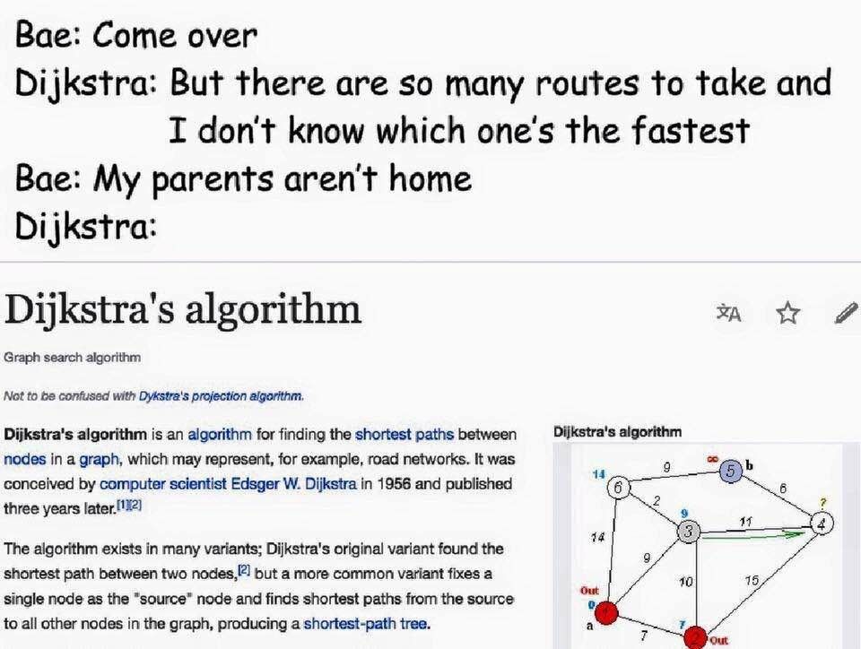
And then follow up on that with the actual backstory from Dijkstra himself:

What is the shortest way to travel from Rotterdam to Groningen, in general: from given city to given city. It is the algorithm for the shortest path, which I designed in about twenty minutes. One morning I was shopping in Amsterdam with my young fiancée, and tired, we sat down on the café terrace to drink a cup of coffee and I was just thinking about whether I could do this, and I then designed the algorithm for the shortest path. As I said, it was a twenty-minute invention. In fact, it was published in '59, three years later. The publication is still readable, it is, in fact, quite nice. One of the reasons that it is so nice was that I designed it without pencil and paper. I learned later that one of the advantages of designing without pencil and paper is that you are almost forced to avoid all avoidable complexities. Eventually, that algorithm became to my great amazement, one of the cornerstones of my fame.

— Edsger Dijkstra, in an interview with Philip L. Frana, Communications of the ACM, 2001

Precondition

As our own naïve algorithm, Dijkstra's algorithm has a precondition that places a requirement of no edges with negative weights in the graph. This precondition is required because of the nature of the algorithm that requires monotonically non-decreasing changes in the costs of shortest paths.

Short description

Let's have a brief look at the pseudocode taken from the Wikipedia:

function Dijkstra(Graph, source):
    for each vertex v in Graph.Vertices:
        dist[v] ← INFINITY
        prev[v] ← UNDEFINED
        add v to Q
    dist[source] ← 0

    while Q is not empty:
        u ← vertex in Q with min dist[u]
        remove u from Q

        for each neighbor v of u still in Q:
            alt ← dist[u] + Graph.Edges(u, v)
            if alt < dist[v]:
                dist[v] ← alt
                prev[v] ← u

    return dist[], prev[]

Dijkstra's algorithm works in such way that it always tries to find the shortest paths from a vertex to which it already has a shortest path. This may result in finding the shortest path to another vertex, or at least some path, till further relaxation.

Given that we need to always choose the cheapest vertex, we can use a min heap to our advantage which can further improve the time complexity of the algorithm.

Used techniques

This algorithm leverages the dynamic programming technique that has already been mentioned with regards to the Bellman-Ford algorithm and also greedy technique. Let's talk about them both!

Dynamic programming technique comes from the fact that we are continuously building on top of the shortest paths that we have found so far. We slowly build the shortest paths from the given source vertex to all other vertices that are reachable.

Greedy technique is utilized in such way that Dijkstra's algorithm always improves the shortest paths from the vertex that is the closest, i.e. it tries extending the shortest path to some vertex by appending an edge, such extended path may (or may not) be the shortest path to another vertex.

Greedy algorithms

Greedy algorithms are algorithms that choose the most optimal action at the moment.

The reason why the algorithm requires no edges with negative weights comes from the fact that it's greedy. By laying the requirement of non-negative weights in the graph we are guaranteed that at any given moment of processing outgoing edges from a vertex, we already have a shortest path to the given vertex. This means that either this is the shortest path, or there is some other vertex that may have a higher cost, but the outgoing edge compensates for it.

Implementation

Firstly we need to have some priority queue wrappers. C++ itself offers functions that can be used for maintaining max heaps. They also have generalized version with any ordering, in our case we need reverse ordering, because we need the min heap.

using pqueue_item_t = std::pair<int, vertex_t>;
using pqueue_t = std::vector<pqueue_item_t>;

auto pushq(pqueue_t& q, pqueue_item_t v) -> void {
  q.push_back(v);
  std::push_heap(q.begin(), q.end(), std::greater<>{});
}

auto popq(pqueue_t& q) -> std::optional<pqueue_item_t> {
  if (q.empty()) {
    return {};
  }

  std::pop_heap(q.begin(), q.end(), std::greater<>{});
  pqueue_item_t top = q.back();
  q.pop_back();

  return std::make_optional(top);
}

And now we can finally move to the actual implementation of the Dijkstra's algorithm:

auto dijkstra(const graph& g, const vertex_t& source)
    -> std::vector<std::vector<int>> {
  // make sure that ‹source› exists
  assert(g.has(source));

  // initialize the distances
  std::vector<std::vector<int>> distances(
      g.height(), std::vector(g.width(), graph::unreachable()));

  // initialize the visited
  std::vector<std::vector<bool>> visited(g.height(),
                                         std::vector(g.width(), false));

  // ‹source› destination denotes the beginning where the cost is 0
  auto [sx, sy] = source;
  distances[sy][sx] = 0;

  pqueue_t priority_queue{std::make_pair(0, source)};
  std::optional<pqueue_item_t> item{};
  while ((item = popq(priority_queue))) {
    auto [cost, u] = *item;
    auto [x, y] = u;

    // we have already found the shortest path
    if (visited[y][x]) {
      continue;
    }
    visited[y][x] = true;

    for (const auto& [dx, dy] : DIRECTIONS) {
      auto v = std::make_pair(x + dx, y + dy);
      auto cost = g.cost(u, v);

      // if we can move to the cell and it's better, relax¹ it and update queue
      if (cost != graph::unreachable() &&
          distances[y][x] + cost < distances[y + dy][x + dx]) {
        distances[y + dy][x + dx] = distances[y][x] + cost;
        pushq(priority_queue, std::make_pair(distances[y + dy][x + dx], v));
      }
    }
  }

  return distances;
}

Time complexity

The time complexity of Dijkstra's algorithm differs based on the backing data structure.

The original implementation doesn't leverage the heap which results in repetitive look up of the “closest” vertex, hence we get the following worst-case time complexity in the Bachmann-Landau notation:

$$\Theta(\vert V \vert^2)$$

If we turn our attention to the backing data structure, we always want the “cheapest” vertex, that's why we can use the min heap, given that we use Fibonacci heap we can achieve the following amortized time complexity:

$$\mathcal{O}(\vert E \vert + \vert V \vert \cdot \log{\vert V \vert})$$

Fibonacci heap

Fibonacci heap is known as the heap that provides $\Theta(1)$ amortized insertion and $\mathcal{O}(\log{n})$ amortized removal of the top (either min or max).

Running the Dijkstra

Let's run our code:

Normal cost: 1
Vortex cost: 5
Graph:
#############
#..#..*.*.**#
##***.....**#
#..########.#
#...###...#.#
#..#...##.#.#
#..#.*.#..#.#
#D...#....#.#
########*.*.#
#S..........#
#############
[Finite BF] Cost: 22
[Bellman-Ford] Cost: 22
[Dijkstra] Cost: 22

OK, so it seems to be working just fine. Now the question arises:

What happens when we have negative weights in our graph?

Busting the myth about looping Dijkstra

One of the very common misconception about Dijkstra's algorithm is that it loops infinitely when you have negative weights or loops in the graph. Well, if we use our propelling vortices, not only we have the negative weights, but also the negative loops. Let's run our code! Our first naïve approach was actually looping:

Normal cost: 1
Vortex cost: -1
Graph:
#############
#..#..*.*.**#
##***.....**#
#..########.#
#...###...#.#
#..#...##.#.#
#..#.*.#..#.#
#D...#....#.#
########*.*.#
#S..........#
#############
[Finite BF] Cost: -240
[Bellman-Ford] Found a negative loop
[Bellman-Ford] Cost: -240
[Dijkstra] Cost: 14

Well, it definitely doesn't loop. How much does 14 make sense is a different matter.

Variations

There are multiple variations of the Dijkstra's algorithm. You can implement it in such way that with negative weights or loops it loops infinitely, but it can be countered. In our case we keep the track of the vertices that already got a shortest path established via the visited, that's how even multiple entries for one vertex in the heap are not an issue.

Summary

Now we have an algorithm for finding the shortest path that is faster than our original naïve brute-force or Bellman-Ford. However we need to keep in mind its requirement of no negative weights for correct functioning.

You can also see how we used our thought process of figuring out the worst-case time complexity for the naïve or Bellman-Ford algorithm to improve the original path-finding algorithms.